Visualizations
(Draft)
Visualizations
For publications, figures (and also tables) form the very first impression to the reader. High quality visualizations are therefore paramount to interest the reader and convey a strong message. In the sections below we provide some starting points when it comes to visualizing data in three dimensions. Pyvista is library designed for fast 3D visualizations and interactive scenes, in a similar vein to vedo and Open3d. While very fast to work with ease of use, the quality of the images is sometimes a tradeoff.
The Mitsuba rendering engine on the other hand is differential rendering library with python bindings. Materials, lighting, subsurface scattering are all modeled, yielding photorealistic images and 3D figures. The cost coming with a rendering engine is the complexity and the need to have a full and deep understanding of materials, how light behaves and what makes a scene good.
In my personal arsenal, both have their place and when used correctly can yield stunning visualizations.
Pyvista
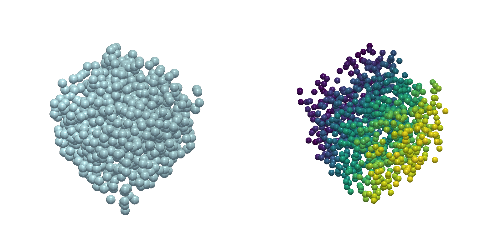
The fastest for proto-typing and animations is pyvista. It runs in a
jupyter notebook and it is very fast to get results. Two unit qubes are
displayed side by side, but any set of point cloud can be rendered. The
line pv.set_jupyter_backend("static") displays the result as a static
image, whereas the option trame yields a pseudo-rendered scene at some
computational cost. If the backend is set to html a very fast
approximation is shown.
import numpy as np
import pyvista as pv
pv.set_jupyter_backend("static")

# Generate random data
first_point_cloud = np.random.uniform(size=(1000,3))
second_point_cloud = np.random.uniform(size=(1000,3))

# Initialize the plotter with two subplots side by side.
# Window size controls the resolution.
pl = pv.Plotter(shape=(1, 2), border=False,window_size=[1600, 800])
pl.subplot(0, 0)
actor = pl.add_points(
    first_point_cloud,
    style="points",
    emissive=False,
    show_scalar_bar=False,
    render_points_as_spheres=True,
    color="lightblue",
    point_size=30,
    ambient=0.2,
    diffuse=0.8,
    specular=0.6,
    specular_power=20,
    smooth_shading=True,
)
pl.subplot(0, 1)
actor = pl.add_points(
    second_point_cloud,
    style="points",
    emissive=False,
    show_scalar_bar=False,
    render_points_as_spheres=True,
    scalars=second_point_cloud[:, 0],
    point_size=20,
    ambient=0.2,
    diffuse=0.8,
    specular=0.8,
    specular_power=40,
    smooth_shading=True,
)

pl.background_color = "w"
pl.link_views()
pl.camera_position = "yz"
pos = pl.camera.position
pl.camera.position = (pos[0], pos[1], pos[2] + 3)
pl.camera.azimuth = -45
pl.camera.elevation = 10
# create a top down light
light = pv.Light(
    position=(0, 0, 3), positional=True, cone_angle=50, exponent=20, intensity=0.2
)
pl.add_light(light)
pl.camera.zoom(1)
pl.show()
For near realtime rendering the quality is great and by setting the resolution higher and subsquently downscaling the image, a quality sufficient for publication can be reached.
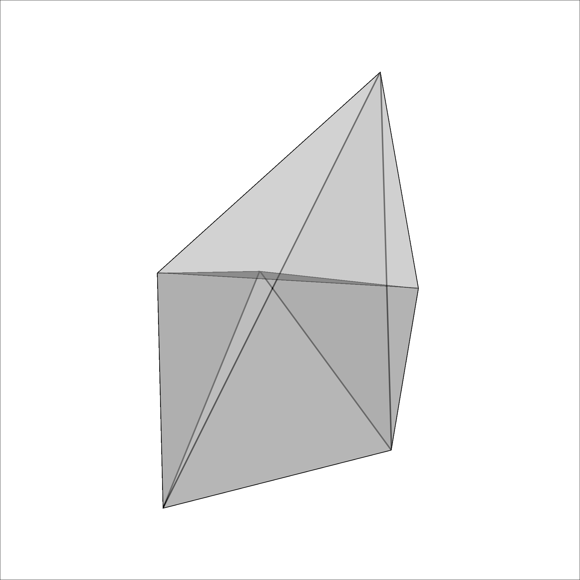
In the next example we will render a triangulation mesh with random node coordinates. First we initialize the data we aim to render.
vertices = np.array([
       [ 0.2770244 , -0.40829167, -0.1979677 ],
       [ 0.2279335 ,  0.66183615,  0.00437725],
       [-0.36964747, -0.5378392 ,  0.00540141],
       [ 0.3479208 ,  0.06662527, -0.1221391 ],
       [-0.09430658,  0.10844991,  0.33278906],
       [-0.38892466,  0.10921948, -0.02246087]], dtype=np.float32)

faces = np.array([
        [0, 0, 0, 0, 1, 1, 2, 3],
        [1, 1, 2, 3, 2, 3, 4, 4],
        [2, 3, 4, 4, 5, 5, 5, 5]])

# Covert the faces to pyvista format mesh.
# [num_vertices, v1, v2, ..., num_vertices, v1,v2,...]
faces_flat = np.hstack(np.vstack([3*np.ones(faces.shape[-1],dtype=int),faces]).T.tolist())
Next we create the mesh and plot it with some opacity.
pl = pv.Plotter(lighting='none',
                     border=True,
                     line_smoothing=True,
                     off_screen=True,
                     window_size=[2000,2000])
light = pv.Light(light_type='headlight')
pl.add_light(light)

# Create the mesh object
mesh = pv.PolyData(vertices, faces_flat)
pl.add_mesh(
    mesh,
    color="lightgray",
    lighting=True,
    show_edges=True,
    line_width=5,
    preference='cell',
    opacity=.8,
    # smooth_shading=True,
)
pl.background_color = 'w'
pl.camera_position = 'xy'
pl.show()
Mitsuba renderer
The Mitsuba renderer is a full fledged rendering engine. We will render the point clouds and the simplicial complex again and it will showcase the complexity.
Each scene in Mitsuba consists of a prefixed set of objects. The
integrator defines how each ray emitted in the scene is tracked on its
path to the sensor, which is the camera. A bsdf is a material, rough
or smooth plastic for instance, which comes with a set of properties. An
emitter is a light source, which emits a type of light.
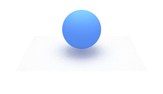
As an illustration, a simple scene with a sphere looks like the following.
import mitsuba as mi
import drjit as dr
from matplotlib import pyplot as plt

mi.set_variant("llvm_ad_rgb")
import numpy as np

COLOR = [0.1, 0.27, 0.86]

scene = mi.load_dict(
    {
        "type": "scene",
        "integrator": {"type": "path"},
        "emitter": {
            "type": "constant",
            "radiance": {
                "type": "rgb",
                "value": [1,1,1],
            },
        },
        "sensor": {
            "type": "perspective",
            "to_world": mi.ScalarTransform4f.look_at(
                origin=[0, 10, 5], target=[0, 0, 0], up=[0, 0, 1]
            ),
            # "fov": 45,
            "film": {
                "type": "hdrfilm",
                "pixel_format": "rgb",
                "width": 1920,
                "height": 1080,
                "rfilter": {
                    "type": "tent",
                },
            },
        },
    'sphere_1': {
          'type': 'sphere',
          'to_world': mi.ScalarTransform4f.scale([1, 1, 1]).translate([0, 0, 1]),
          "material": {
                    "type": "diffuse",
                    "reflectance": {"type": "rgb", "value": COLOR},
                },
      },
        "ground_plane": {
            "type": "rectangle",
            "to_world": mi.ScalarTransform4f.translate([0, 0, -0.25]).scale([3, 2, 1]),
            "material": {
                "type": "diffuse",
                "reflectance": {
                    "type": "rgb",
                    "value": 0.75,
                },
            },
        },
        "emitter_plane": {
            "type": "rectangle",
            "to_world": mi.ScalarTransform4f.translate([0, 0.0, 5])
            .scale(2.0)
            .rotate([1, 0, 0], 2.0),
            "flip_normals": True,
            "emitter": {
                "type": "area",
                "radiance": {
                    "type": "rgb",
                    "value": 5,
                },
            },
        },
    }
)

img = mi.render(scene, spp=8)
plt.axis("off")
plt.imshow(mi.util.convert_to_bitmap(img))
The next section will go over each component in the scene.
Integrator
Defaults to path type integrator and can be left on default for most purposes.
Sensor
The sensor is the camera and the location of the camera is controlled
with the to_world transform. The origin is where the camera is located
and the target is what the camera looks at.
Emitters
In this scene there are two emitters (lights), the first is constant emitter that provides a global illumination, as a room. The color is controlled with the rgb values. The second emitter is a plane that creates the shadow. The plane is located above the scene and the flipped normals ensure that the light shines down onto the scene. A diffuse shadow is created since the light is emitted from each point in the plane, the size of the plane controls the sharpness of the plane.
Shpere and ground plane
The ground plane is a light gray material with a diffuse type material that makes the ground non-reflective. For the material of the sphere we also use a diffuse material with a blue color.
Rendering
The spp (samples per pixel) argument in the render command at the end
controls how high the quality of the render is, at the cost of time.
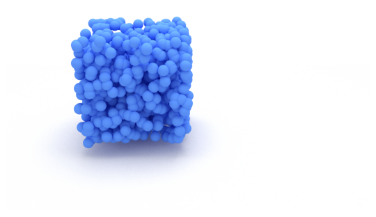
Render a point cloud
We will render the same point clouds as with Pyvista. The difference is
that we will have to place each shpere “by hand” in the scene, create
the lighting and set up the camera, which was all accounted for my
pyvista. The ground plane is set at z=0 and the unit cube is added on
top.
import numpy as np
import mitsuba as mi
import drjit as dr
from matplotlib import pyplot as plt

mi.set_variant("llvm_ad_rgb")


# Generate random data
point_cloud = np.random.uniform(size=(1000,3))

pc_dict = {}
for idx, point in enumerate(point_cloud):
    x,y,z = point
    pc_dict[f"point_{idx}"] = { 'type': 'sphere',
                               'radius':.05,
        'to_world': mi.ScalarTransform4f.translate([x, y, z]),
        "material": {
                  "type": "diffuse",
                  "reflectance": {"type": "rgb", "value": COLOR},
              }
      }

COLOR = [0.1, 0.27, 0.86]
#
scene = mi.load_dict(
    {
        "type": "scene",
        "integrator": {"type": "path"},
        "emitter": {
            "type": "constant",
            "radiance": {
                "type": "rgb",
                "value": [1,1,1],
            },
        },
        "sensor": {
            "type": "perspective",
            "to_world": mi.ScalarTransform4f.look_at(
                origin=[0, 5, 2], target=[0, 0, 0], up=[0, 0, 1]
            ),
            # "fov": 45,
            "film": {
                "type": "hdrfilm",
                "pixel_format": "rgb",
                "width": 2*1920,
                "height": 2*1080,
                "rfilter": {
                    "type": "tent",
                },
            },
        },
        "ground_plane": {
            "type": "rectangle",
            "to_world": mi.ScalarTransform4f.translate([0, 0, -0.1]).scale([3, 2, 1]),
            "material": {
                "type": "diffuse",
                "reflectance": {
                    "type": "rgb",
                    "value": 0.75,
                },
            },
        },
        **pc_dict,
        "emitter_plane": {
            "type": "rectangle",
            "to_world": mi.ScalarTransform4f.translate([0, 0.0, 5])
            .scale(2.0)
            .rotate([1, 0, 0], 2.0),
            "flip_normals": True,
            "emitter": {
                "type": "area",
                "radiance": {
                    "type": "rgb",
                    "value": 5,
                },
            },
        },
    }
)

img = mi.render(scene, spp=64)
plt.axis("off")
plt.imshow(mi.util.convert_to_bitmap(img))